How to annotate in Roboflow
When training a YOLO model, it is important to make good annotations for your images. To make annotating easier, you can use Roboflow.
To get started, create an account. You can choose to log in with Github aswell. When creating an account, you can get a 30-day trial of the premium features, but for basic annotations these are not necessary.
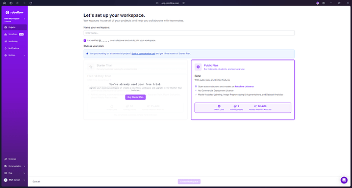
When you have created an account, you can create a workspace with the name of your project from the menubar on the left. Once you have created a workspace, you can add other members to collaborate on annotating. Be aware that you can only have 3 members in a workspace on the free tier of roboflow and your project will be public.
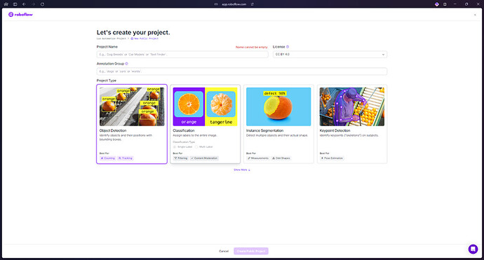
When your workspace is created, you can create one or more projects inside the workspace. When creating your project, you need to decide what type of detection you want to train.
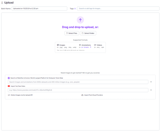
Once you have created a project, you can start adding images of your object(s) from the upload data tab on the left side of the screen. Make sure your files are in the supported formats.
You can choose to manually label the images, auto label them or get strangers to do it through roboflow. For the rest of this how-to I assume you are going to annotate manually.
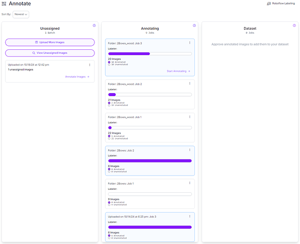
When you have uploaded data, the images can be assigned to specific people in your workspace.
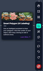
Depending on the complexity of your object and environment of the image you can choose to annotate with square bounding boxes or polygons. When annotating bounding boxes on more compIex objects I would recommend using the smart polygon tool.
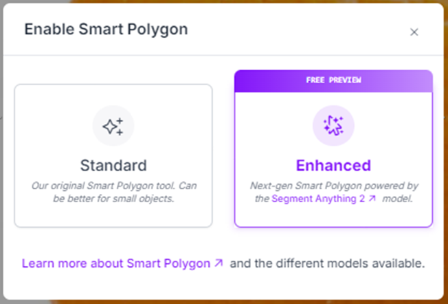
Clicking on the smart polygon tool gives this popup.
With the standard smart polygon tool, you can either click on the object, hold the mouse button and drag a square around the object. With the advanced smart polygon tool you can hover over the object, and the automatically detected object will be highlighted, then selected when you click.
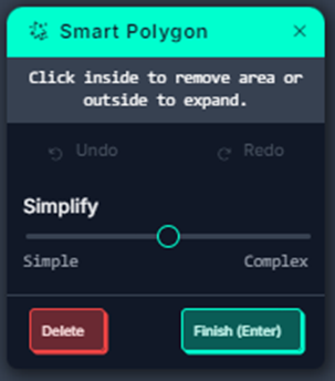
Depending on the complexity of the object, you can drag the slider on the popup after marking the object. This will increase or decrease the amount of points of the polygon.
When clicking finish on the popup, you can name the class of object and edit the position of the polygon points if you want to. If you already have classes made, you can pick from the list.
If you have multiple images, you can switch between them in the top of the screen.
After annotating all the objects in your image(s), simply go back and the images have been marked as annotated. They can now be added to the dataset from the top right corner of the annotate tab. You can decide how the annotated images should be split between training/validation/test pools.
You can now see all the data in the dataset from the dataset tab.
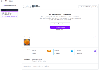
Once you are ready to download your dataset, head to the generate tab. Here you can add preprocessing and augmentation to your dataset and create the downloadable file.
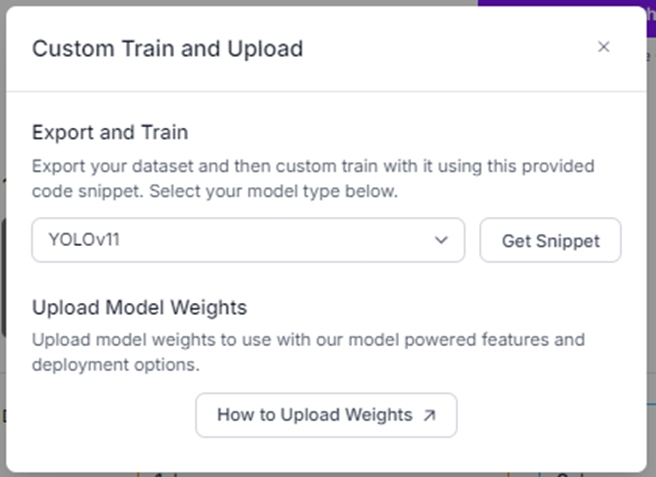
From this screen you should click custom train and upload.
Then pick the correct formatting for your YOLO version. If you see a checkbox to train on roboflow, uncheck it.
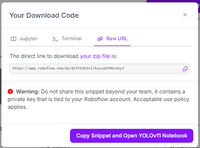
Your dataset is now ready to be downloaded. You can use it in multiple ways, including downloading a zip file by clicking on your zip file.
Unzip the file, and copy the path of the included data.yaml file.
To train your yolomodel on the dataset, open the command prompt (press WIN + X then I or search cmd in the start menu), and use this command
yolo task=detect mode=train data=path/to/bounding_box_dataset.yaml model=yolov8n.pt epochs=100 imgsz=640If you get an error about “OMP: OpenMP runtime”, use this command and try again.
set KMP_DUPLICATE_LIB_OK=TRUE If you another version of YOLO, change the model to the correct version.
epochsis the number of iterations for the training andimgszis the pixel size of the images.
If you want to train keypoints use this command instead
yolo task=pose mode=train data=path/to/keypoint_dataset.yaml model=yolov8n-pose.pt epochs=100 imgsz=640
The training will take a while depending on your hardware and dataset.
When the training is done, the terminal will tell you where the run is saved. The default save path is user\runs\detect\trainX for bounding boxes and user\runs\pose\trainX for keypoints.
If the training is completed without error, the folder should look something like this
You can now load the path_to_train\weights\best.pt into your python script and use the trained model to analyze images etc.
